Yr12 Journal 4

In week 6 I learned about multivariable linear regression.

The concept

Multivariable linear regression is similar to what I did last week, the basic linear regression, the only different is in this case it has multiple independent variables that will affect the output, hence there comes out a maths function to calculate the coefficients of a linear equation that describes the destribution of the data (with different independent variables).

Why we doing this

To let the machine gain the ability to make accurate predictions, it needs to learn from accurate data. However, most data have various independent variables that will affect the output, hence multivariable linear regression is needed to find out the linear relationship between various inputs and the output, so then with different inputs the machine can give highly accurate response.

How I went

• I successfully run the code provided in the Google Docs with the provided data
• When I was trying to implement my multivariable linear regression with my data, I found some bugs, so I fixed them.
  • ie. the length of the X was limited to 47 when it comes to compute cost or to plot, this leads to a disaster when there are more or less than 47 entrieds of data provided.
  • While sorting data, it is essential to drop all nan in the dataframe otherwise when it comes to calculation errors will occur.

What I did

I did a PM2.5 and PM2.5/hr vs AQI_PM2.5 linear regression analyse. I collected the data from ACT Open Data Portal and I implemented it as following:

import numpy as np
import pandas as pd
import matplotlib.pyplot as plt
from tqdm import tqdm

epoch = 1000
rate = 0.01

max = 1000
col1 = "PM2.5"
col2 = "PM2.5 1 hr"
col3 = "AQI_PM2.5"
df = pd.read_csv('Air_Quality_Monitoring_Data.csv')
df = df[[col1, col2, col3]]
print(f"{len(df)} entries of data")
df = df.dropna()
print(df.dtypes)
m = len(df)
max = max if max <= m else m
m = max
df = df.iloc[:m, :]
df.columns = range(df.shape[1])
print(f"{len(df)} entries selected")
np.seterr('raise')
print(df.head())

df = pd.concat([pd.Series(1, index=df.index, name='00'), df], axis=1)
print(df.head())

X = df.drop(columns=2)
y = df.iloc[:, 3]


theta = np.array([0.0] * len(X.columns))
m = len(df)


def hypothesis(theta, X):
    return theta * X


def computeCost(X, y, theta):
    y1 = hypothesis(theta, X)
    y1 = np.sum(y1, axis=1)
    return sum(np.sqrt((y1 - y) ** 2)) / (2 * m)


def gradientDescent(X, y, theta, alpha, i):
    J = []  # cost function in each iterations
    k = 0
    pbar = tqdm(total=i)
    while k < i:
        y1 = hypothesis(theta, X)
        y1 = np.sum(y1, axis=1)
        for c in range(0, len(X.columns)):
            theta[c] -= alpha * (sum((y1 - y) * X.iloc[:, c]) / len(X))
        j = computeCost(X, y, theta)
        J.append(j)
        k += 1
        pbar.update(1)
    return J, j, theta


J, j, theta = gradientDescent(X, y, theta, rate, epoch)
y_hat = hypothesis(theta, X)
y_hat = np.sum(y_hat, axis=1)

plt.figure()
plt.scatter(x=list(range(0, m)), y=y, color='blue', label='original y')
plt.scatter(x=list(range(0, m)), y=y_hat, color='black', label='prediction')
plt.legend(loc = "upper right")
plt.xlabel("epoch")
plt.ylabel("original and predicted Output")
plt.show()

plt.figure()
plt.scatter(x=list(range(0, epoch)), y=J)
plt.xlabel("epoch")
plt.ylabel("cost")
plt.show()
print(theta)

I did 1000 epoches on 1000 data with a rate of 0.01 otherwise it will take too long for my laptop to process.

Results

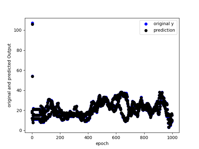
• My coefficients: [-0.10525957 3.93943139 -0.00469064]

• Original vs Prediction:

  

  As it shows it is really accurate as most the predictions overlap the original values.

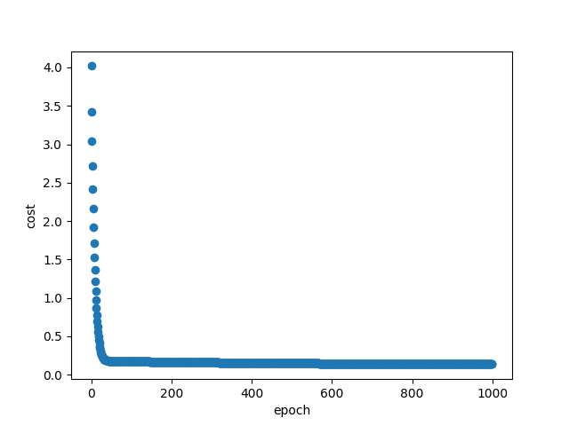
• Cost of the linear regression:

  

  Again the cost supports that the confidence of the calculated coefficients, as they are really accurate.

Conclusion

Everything went well this week, I learned some maths and I leanred how to implement linear regression. And I successfully analysed the distribution of the data I provided.