
In Term 3 Week 2, I was working on my project.
Although it says this blog post has a word count more than 1000 words, it includes the code count as well, so the actual blog post is less than 1000 words
Progress
I have to apologise to myself. I underestimated myself. Although I planeed to spend 3 weeks on data crawling, model training and model implementation, I finished all of these on Saturday afternoon with a cup of coffee. The progress was more successful than I though it would be. Therefore I feel sorry to myself such that I would plan to spend that long time on such simple things.
First of all, let’s discuss what have I done on Saturday
Data Crawling
Of course this Data Science needs data to work, so do my project. My project requires a heaps of accurate market data, and fortunately Binance Crypto Market has API that provides all I need, it provides:
K-Line Data in a specefic range of time with the specefic interval
1
2
3
4
5
6
7
8
9
10
11
12
13
14
15
16
[
[
1499040000000, // Open time
"0.01634790", // Open
"0.80000000", // High
"0.01575800", // Low
"0.01577100", // Close
"148976.11427815", // Volume
1499644799999, // Close time
"2434.19055334", // Quote asset volume
308, // Number of trades
"1756.87402397", // Taker buy base asset volume
"28.46694368", // Taker buy quote asset volume
"17928899.62484339" // Ignore.
]
]Basically I can use this to get all price/number of trades/volume/time in a given range, I can use this data to train a model. Alternatively, I can use this API to get recent data and input this to the model and get a output price
Current Avg Price of a specefic coin one other (i.e. ETH to BTC, or even BTC to AUD)
1
2
3
4
{
"mins": 5,
"price": "9.35751834"
}Basically I can get the price of the coin at current time, and apply it to a trained model to predict the price in the future
As we can see, I have got lots of useful, accurate, and complete data, at any time period.
Now I need to combine those data in a period of time to a DataFrame so we can use it to train a model.
After overtake a few Challenges, here is the code for data crawling process:
1 | def get_history_df(coin, year, month): |
where:
1 | def get_certain_time(year, month, day, hour, min): |
1 | def get_k_for_coin(name, start, end): |
1 | def get_k_for_BTC_baseline(start, end): |
1 | def get_dataframe_from_kline(coin_kline, btc_kline): |
By doing this, now we have a DataFrame that contains the
- ‘Open Time Hr’
- ‘Open’
- ‘High’
- ‘Low’
- ‘Volume’
- ‘Close Time Hr’
- ‘Quote Asset Volume’
- ‘Trades’
- ‘Buy Base’
- ‘Buy Quote’
- ‘BTC Open’
- ‘BTC High’
- ‘BTC Low’
- ‘BTC Close’
- ‘BTC Volume’
- ‘BTC Trades’
- ‘Close Price’
In a given time. These are the factors I think that have a correlation to the close price.1
2
3
4
5
6
7
8
9
10
11
12Open Time Hr Open High ... BTC Close BTC Volume BTC Trades
33853 12 0.069273 0.069325 ... 31804.65 0.10191 4.0
34303 21 0.070211 0.070212 ... 31761.30 0.12436 9.0
20758 1 0.058891 0.058891 ... 30723.81 0.27317 18.0
28130 9 0.065255 0.065255 ... 33826.62 0.19866 6.0
32476 12 0.069774 0.069780 ... 32410.61 0.07023 10.0
... ... ... ... ... ... ... ...
30427 1 0.067749 0.067758 ... 33662.69 0.28920 11.0
13101 11 0.056726 0.056726 ... 31262.10 0.17775 7.0
13547 18 0.055691 0.055708 ... 31100.57 0.05177 7.0
4982 14 0.055103 0.055122 ... 28014.05 0.20659 16.0
20193 14 0.058244 0.058287 ... 30487.53 0.04745 8.0
Model Training
I used Tensorflow to train my model, I split my data as input and output.
- Input has 16 variables (the first 16 facotrs mentioned above)
- Output has 1 variable (Close Price)
I also normalised all the data to make it easier to train (z-score method), to be able to reverse the operation and make prediction of current price, reverse normalised process is also required:
1 | def get_norm_df(df): |
I split my data as 80% training data and 20% testing data, also I split the input and output:
1 | def get_train_dataset(df: DataFrame): |
As now I have all the data I need, I can crate my model:
1 | def create_model(train_dataset: DataFrame): |
I will explain why I chose to make a Sequential Model and why I had these params in the next blog post, due to the word limit.
Just a brief description, I build a model that has 3 layers, input layer (with 16 inputs, or train_dataset.keys().length inputs), and I have a hidden layer (with 16 units), finally I have an output layer that output one unit. I have a learning rate of 0.0005 (tried a whole afternoon and figure out this number gives the most accurate result). Finally I used Mean Absolute Error and Mean Square Error to calculate the loss as a metrics.
Lets see the result:
1 | Model: "sequential" |
1 | loss mae mse ... val_mae val_mse epoch |
1 | Testing set Mean Abs Error: 0.01 Close Price |
As we can see, the error is 0.01 of the normalised price, this is very accurate!
Lets compare the test output and the predicted output:
- Test output
1
[-1.22100359 -1.21980964 -1.20701729 ... 1.44731059 1.46180858 1.52031228]
- Predicted output
1
[-1.2320391 -1.2223128 -1.2007444 ... 1.4353155 1.4469447 1.5193961]
It is amazingly accurate!
Let’s have a look on some plots:
Mean Absolute Error

Mean Square Error

Actual Output v.s. Prediction

In conclusion I trained an accurate model
Model Implementation
I used it to predict the price of a coin in the next 60 minutes with the following code:
1 | coin = "ETH" |
where:
1 | def download_last_hr_data(coin): |
1 | def plot(coin, indexes, mins): |
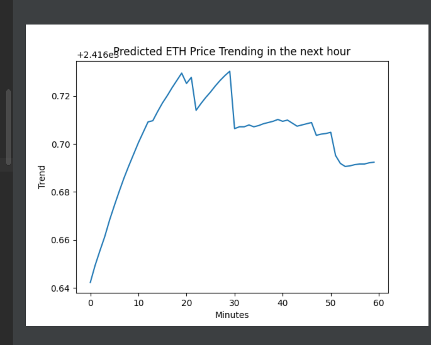
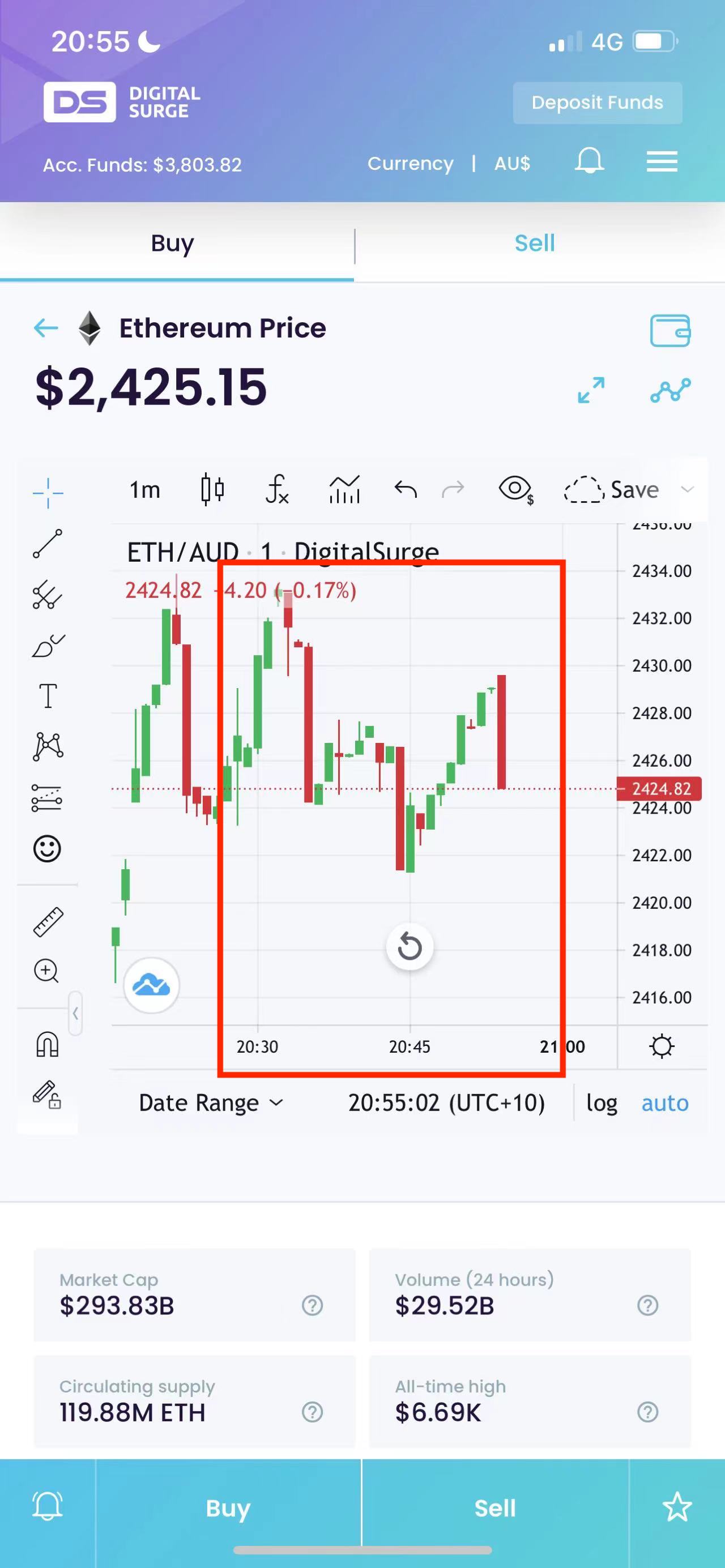
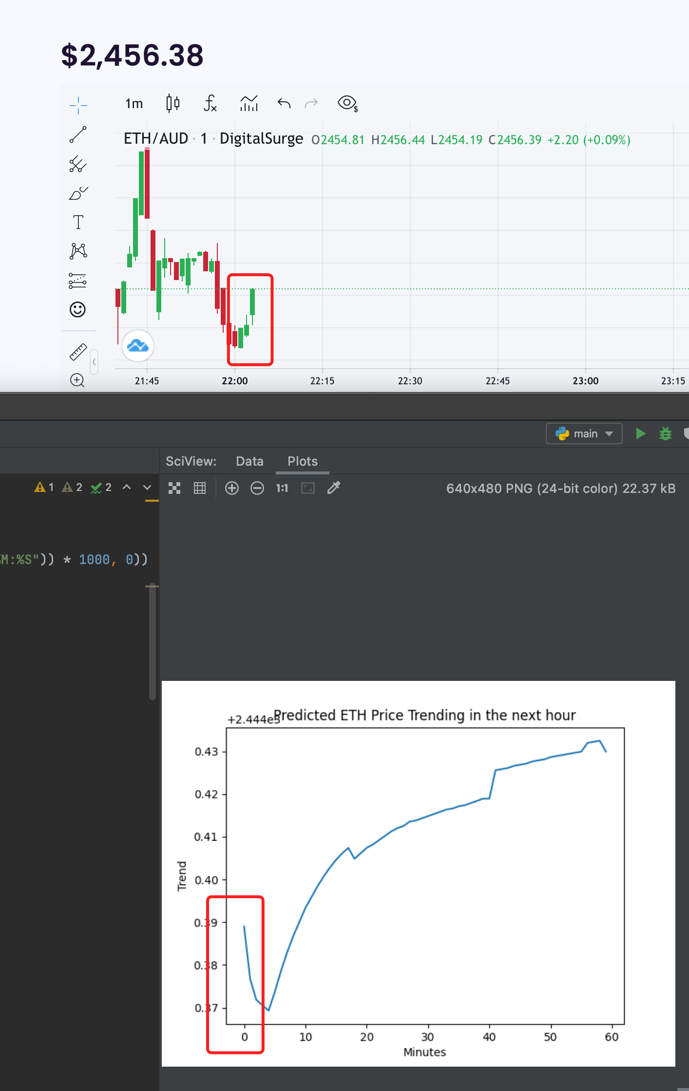
And here is a sample result:

The trending is unbelievable accurate as I spent my whole Saturday night testing it:
Saturday 8.30pm test
Saturday 9.05pm test
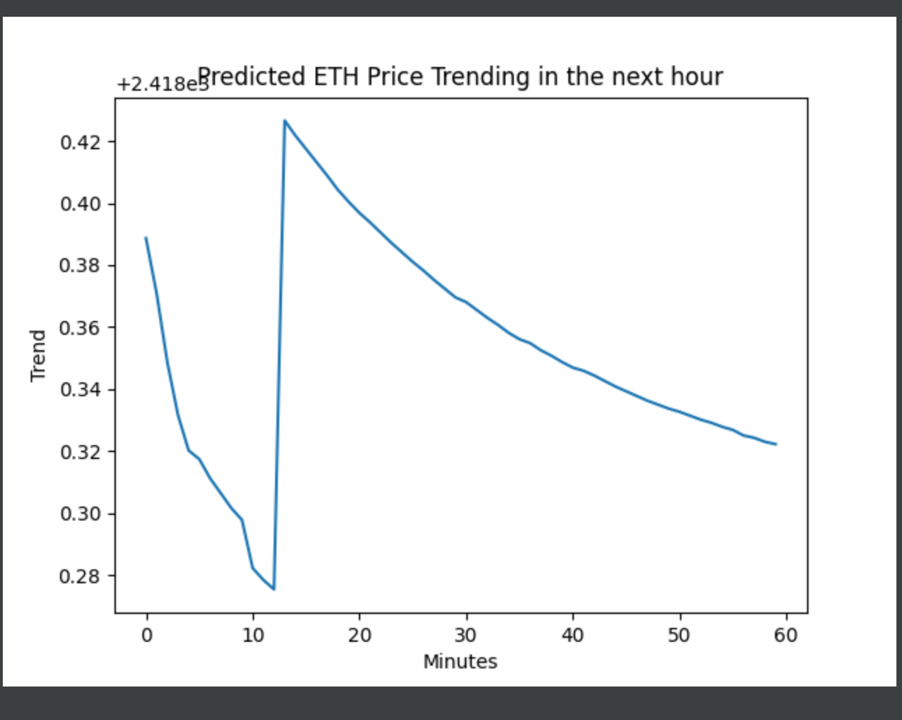
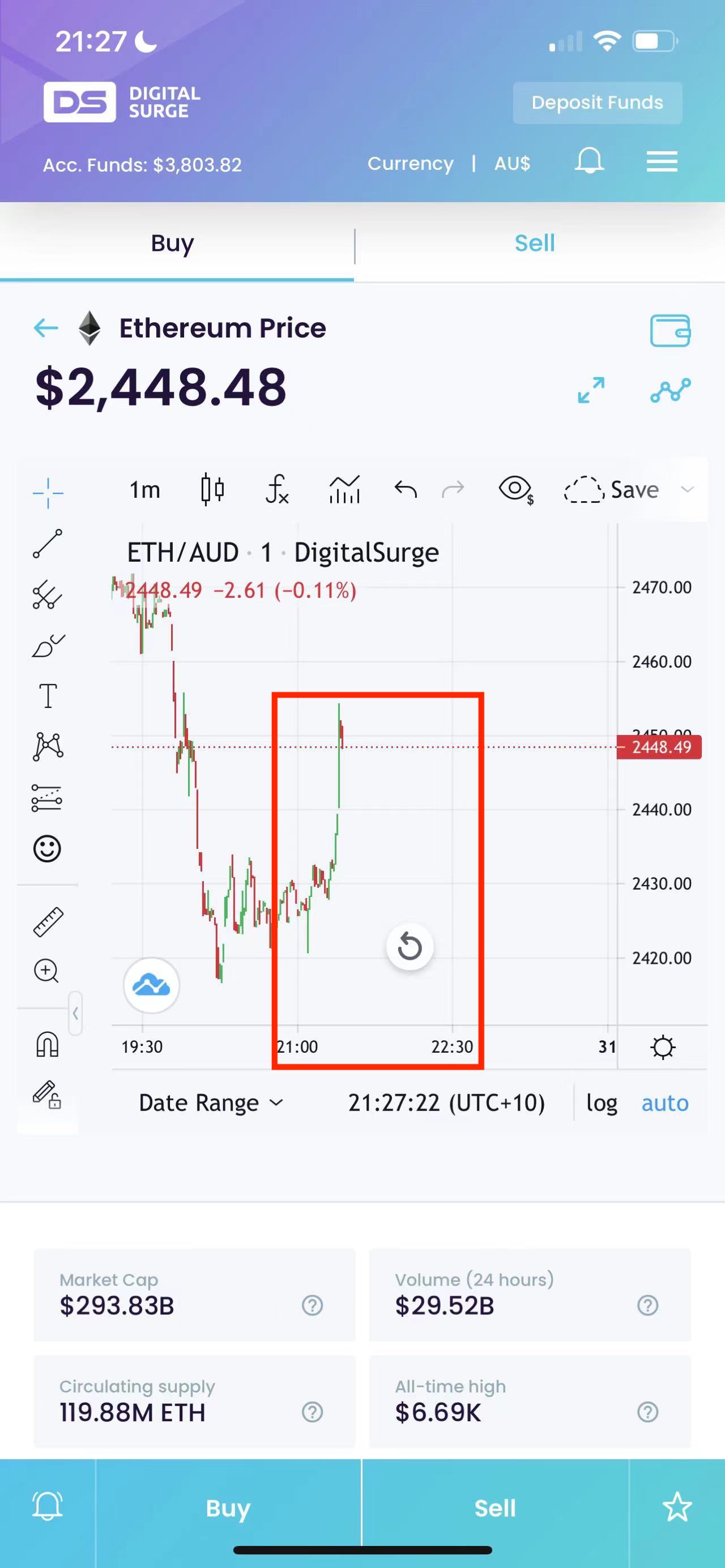
Saturday 10pm test
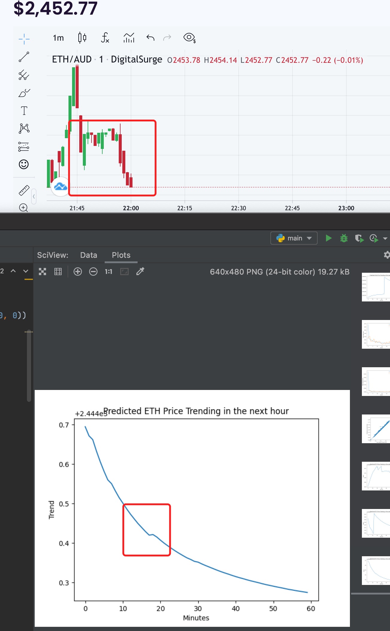
Saturday 11pm test
Challenges
- Binance K Line API only return 1000 entries per request
To overtake this, I have to split my requests, I requested 600 entries per time (600 minutes’ data -> 10 hrs’ data), and I requested mutiple times, to get the 24 hour data in a specefic day. - Binance K Line API needs to input date manually
I made a for loop that iterates day 1 to day 28 in a month, and gets the 24 hour data on that day. (In the future I will let the program figure out how many days are there exactly in a given month). - As Tensorflow does not support using Mac GPU to train model (although I have a Radeon Pro Vega 20 4 GB Graphic Card), I have to use CPU to train model, and this is really slow. Therefore I reduced the layers and units of my model to increase the training speed. Also I implemented an early stop callback, when the loss is approximately the same for 10 epoches, then stop the training process.
Reflection
- I learned how to use Tensorflow and to train a model using a given data, and how to evaluate and predict output.
- I learned how the basics of Machine Learning Process works, I will explain this in the next blog post due to word count limit
- I have done everything well this week.
Timeline
I am on track, and I am too beyond. I finished all the work I planned to work on for the first three weeks. I might need to change my timeline, because I believe I can finish the User Interface next week, therefore I have extra few weeks to spend on testing. Hence, I think I will spend around 8 weeks on testing the accuracy and validity of the model.
I planned to design a GUI for my project next week, so users can choose whatever coin they want to train and predict, also they can specify a range of time of the data they want to use to train the model. Also I planned to finish my User Document and my Presentation PowerPoint.